
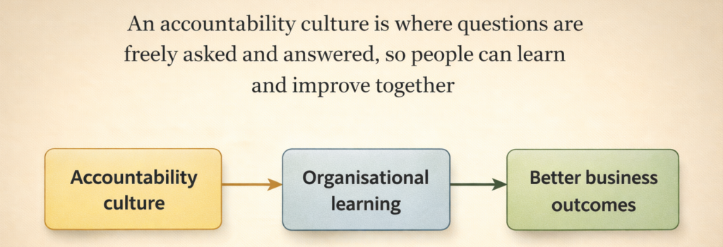
In Unaccountability is how organisations fail to improve, I talked about how becoming a learning organisation is the pathway to better business outcomes, and why unaccountability prevents learning. I’ve been thinking about hindsight bias recently, and why it’s different to an unaccountability culture. Unlike unaccountability, hindsight bias isn’t a choice, and it’s universal.
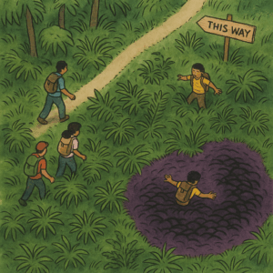
Hindsight bias is when perceptions of today impair perceptions of yesterday. It strips away the rich context behind decisions. It makes answers seem obvious. A candidate withdraws from a hiring process – they weren’t the right fit for us. A client ends a contract – they were never the right partner for us. A system is launched on time – they were always going to hit the deadline. Hindsight bias is unfair, and it’s unhelpful.
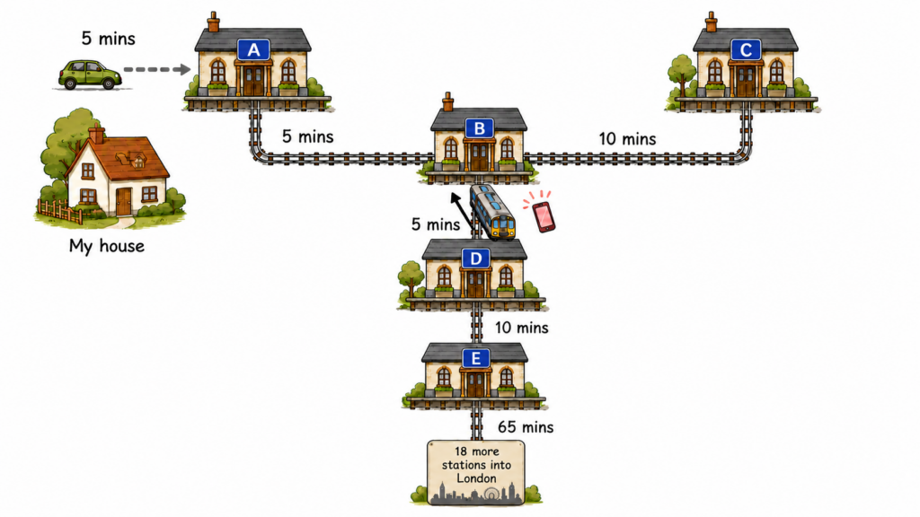
Trains, phones, and automobiles
I had a great example of hindsight bias recently, when a friend contacted me to say they’d left their iPhone on a train headed into London. When I logged into Find My, I was surprised to see the iPhone was headed back from London, and it was near station B. An app showed the train’s destination was my local station, so I drove to station A.
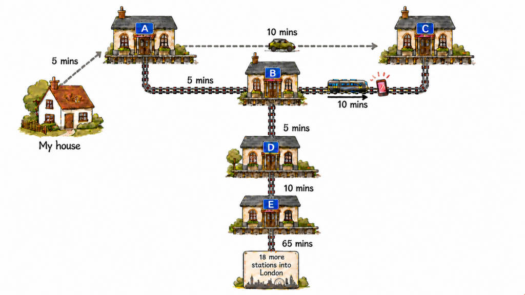
At station A, the train was due, but Find My suddenly showed the iPhone headed towards station C. The train had changed destination! So I asked station A staff to phone station C and search the train, and I drove there.
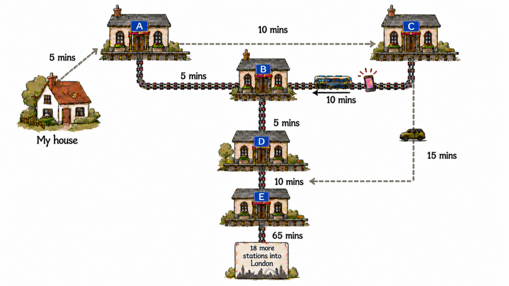
At station C, the train departed back to London just as I arrived. Staff hadn’t found a phone, but Find My updated to show the iPhone headed back to station B! So I asked station C staff to phone station D to search the train, and I started to drive there… until I parked the car and thought: this is silly, I can’t race a train, station staff won’t find the iPhone, I’ll drive home and file a lost property report.
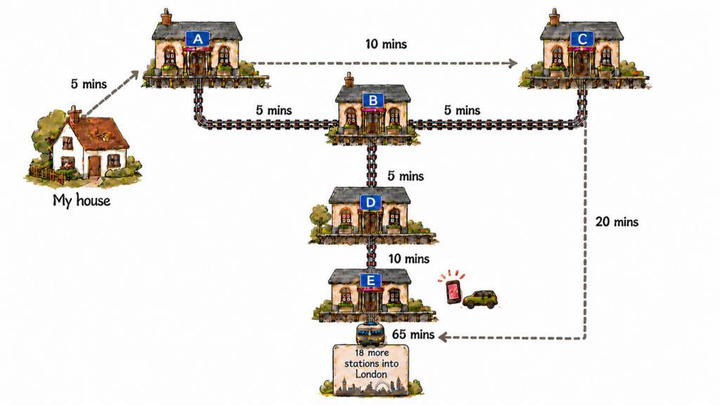
But as I turned for home, Find My updated to show the phone stationary at station E – not station D as hoped! So I drove to station E, where the staff said (deep breath) station D staff had phoned to say station C staff had phoned to say station A staff had phoned to say search for an iPhone. And they had the phone, so I said thanks, wrote a positive feedback form, and then drove home to resume work.
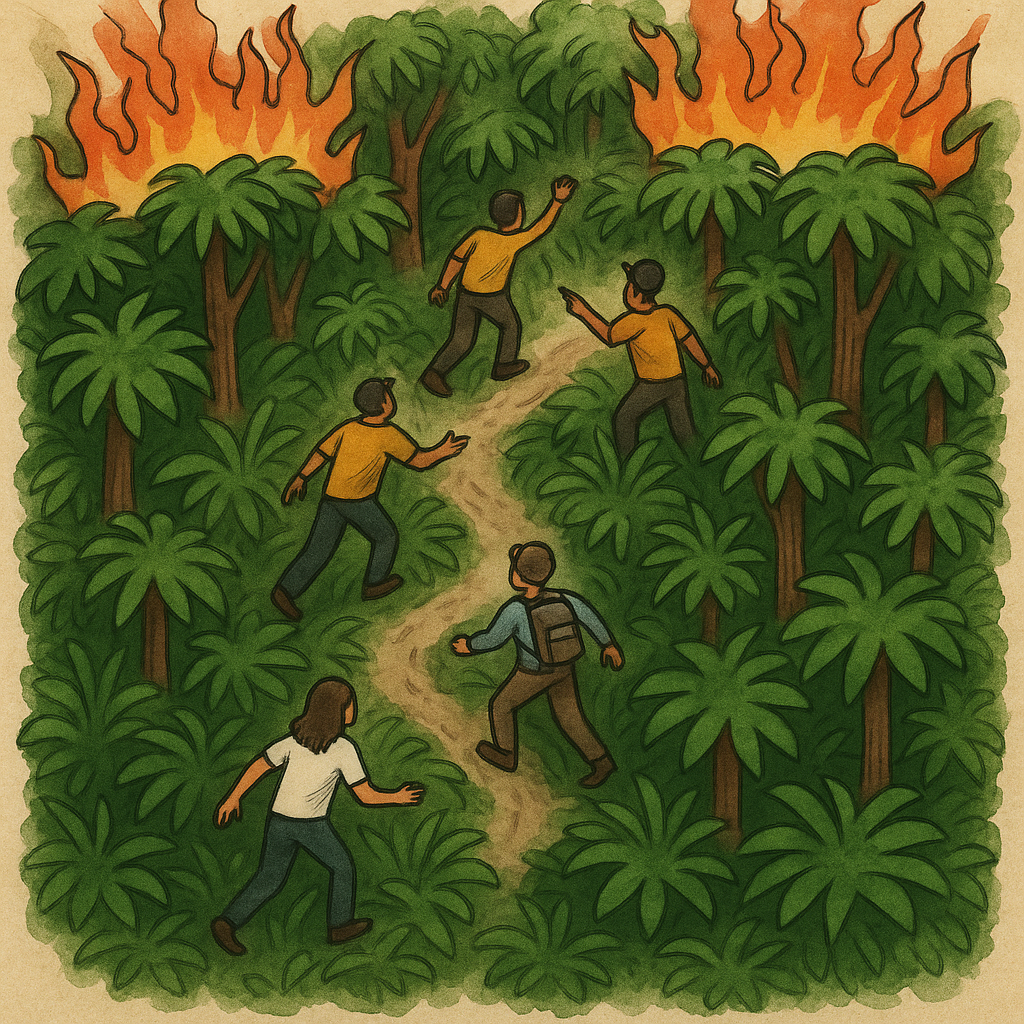
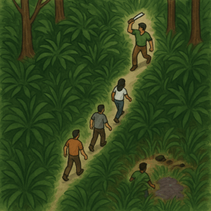
Hindsight bias kills context
In hindsight, it’s obvious what I should have done. At the outset, I should have driven from my house to station B, and waited for the iPhone to go to station A or C, then come back to station B on the same train. Let the iPhone come to me in 10 mins, not chase it for 60. Except… it’s not obvious when you’re inside the problem. I was driving a car, watching Find My updates, wondering about iPhone backups, and making fast decisions with slow data.
Understanding the context in which outcomes happened is where the value is. It’s never as simple as the candidate was the wrong fit, or the client was the wrong partner, or the system was always going to be launched on time. In my case, it wasn’t as simple as just drive to station B. There were lots of surprises to learn from – Find My updates can be slow, trains can change destination at the end of the line, and station staff can be very kind.
Acknowledgement of hindsight, and curiosity about context, is essential if learning is going to happen.
Thanks to Amelia Bampton Jon Ayre Saqib Afghan and Sarah Farrington for their feedback on this.
Recent Comments