On Tech

Tag: Pipeline

Deployment pipeline design and the Theory Of Constraints

How should you design a deployment pipeline? Short and wide, long and thin, or something else? Can you use a Theory Of Constraints lens to explain why pipeline flexibility is more important than any particular pipeline design?

TL;DR:

  • Past advice from the Continuous Delivery community to favour short and wide deployment pipelines over long and thin pipelines was flawed
  • Parallelising activities between code commit and production in a short and wide deployment pipeline is unlikely to achieve a target lead time 
  • Flexible pipelines allow for experimentation until a Goldilocks deployment pipeline can be found, which makes Continuous Delivery easier to implement

Introduction

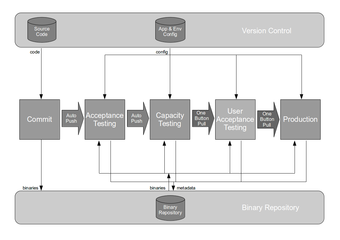
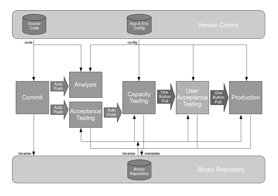
The Deployment Pipeline pattern is at the heart of Continuous Delivery. A deployment pipeline is a pull-based automated toolchain, used from code commit to production. The design of a deployment pipeline should be aligned with Conway’s Law, and a model of the underlying technology value stream. In other words, it should encompass the build, testing, and operational activities required to launch new product ideas to customers. The exact tools used are of little consequence.

Advice on deployment pipeline design has remained largely unchanged since 2010, when Jez Humble recommended “make your pipeline wide, not long… and parallelise each stage as much as you can“. A long and thin deployment pipeline of sequential activities is easy to reason about, but in theory parallelising activities between build and production will shorten lead times, and accelerate feedback loops. The trade-off is an increase in toolchain complexity and coordination costs between different teams participating in the technology value stream.

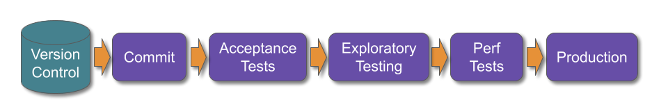
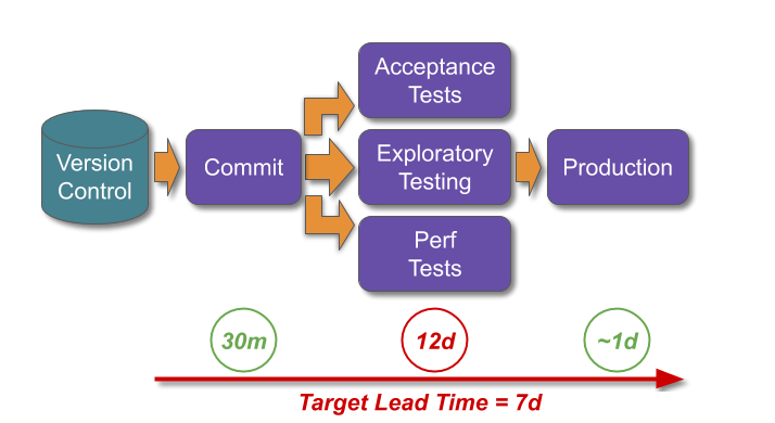
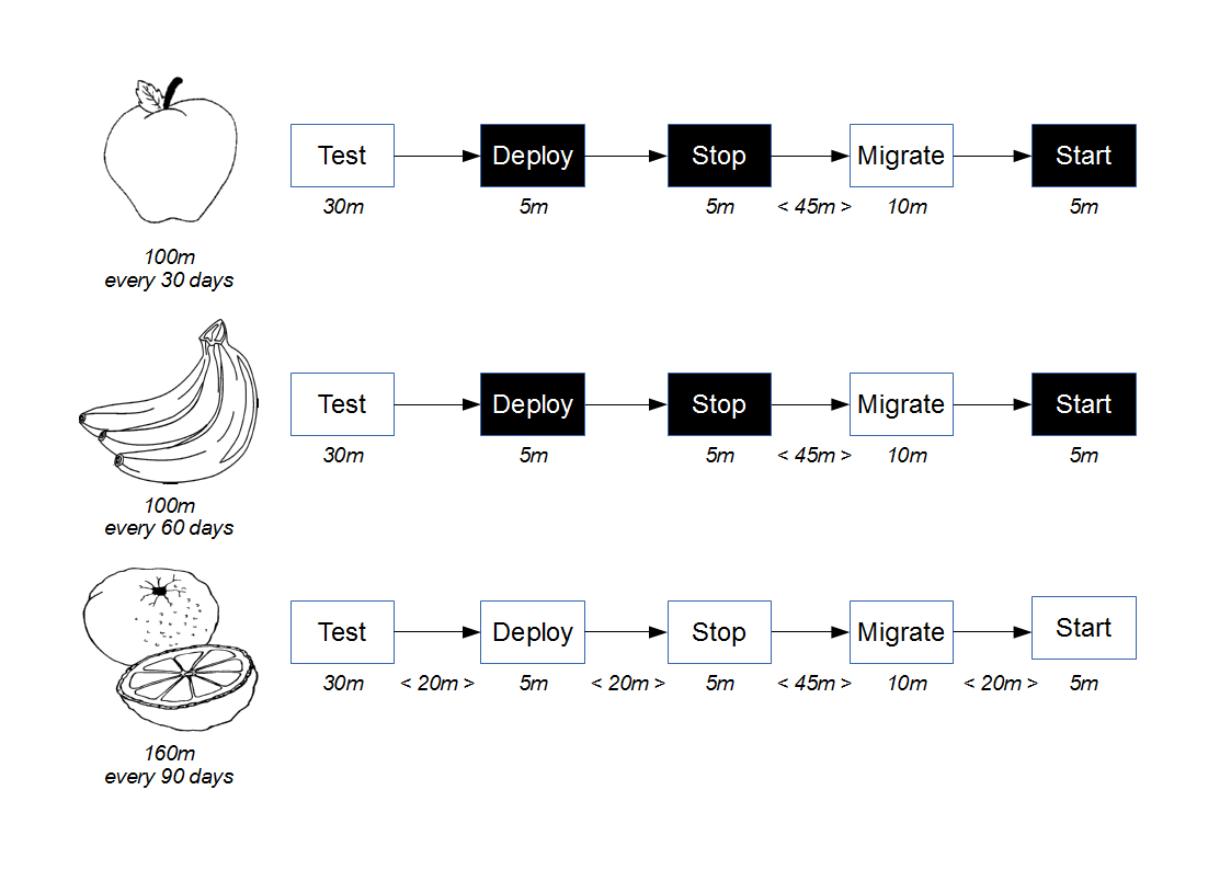
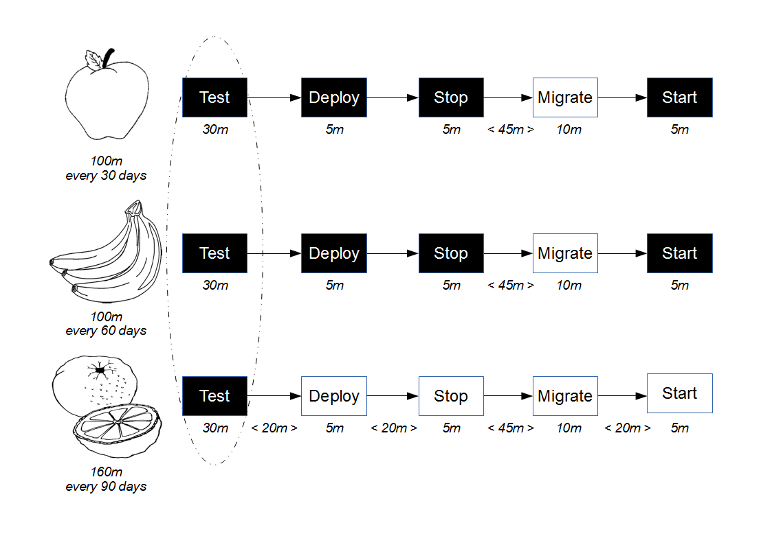
For example, imagine a technology value stream with sequential activities for automated acceptance tests, exploratory testing, and manual performance testing. This could be modelled as a long and thin deployment pipeline.

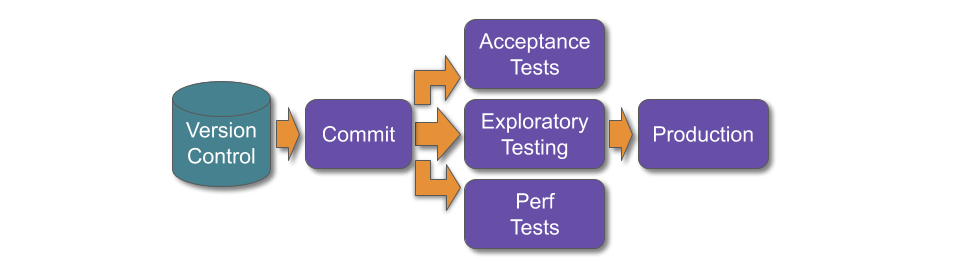
If those testing activities could be run in parallel, the long and thin deployment pipeline could be re-designed as a short and wide deployment pipeline.

Since 2010, people in the Continuous Delivery community – including the author – have periodically recommended short and wide deployment pipelines over long and thin pipelines. That advice was flawed.

The Theory Of Constraints, Applied

The Theory Of Constraints is a management paradigm by Dr. Eli Goldratt, for improving organisational throughput in a homogeneous workflow. A constraint is any resource with capacity equal to, or less than market demand. Its level of utilisation will limit the utilisation of other resources. The aim is to iteratively increase the capacity of a constraint, until the flow of items can be balanced according to demand. The Theory Of Constraints is applicable to Continuous Delivery, as a technology value stream should be a homogeneous workflow that is as deterministic and invariable as possible.

When a delivery team is in a state of Discontinuous Delivery, its technology value stream will contain a constrained activity with a duration less than the current lead time, but too large for the target lead time. The duration might be greater than the target lead time, or the largest duration of all the activities. A short and wide deployment pipeline will not be able to meet the target lead time, as the duration of the parallel activities will be limited by the constrained activity.

In the above example, assume the current lead time is 14 days, and manual performance testing takes 12 days as it involves end-to-end performance testing with a third party.

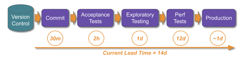
Assume customer demand results in a target lead time of 7 days. This means the delivery team are in a state of Discontinuous Delivery, and a long and thin deployment pipeline would be unable to meet that target.

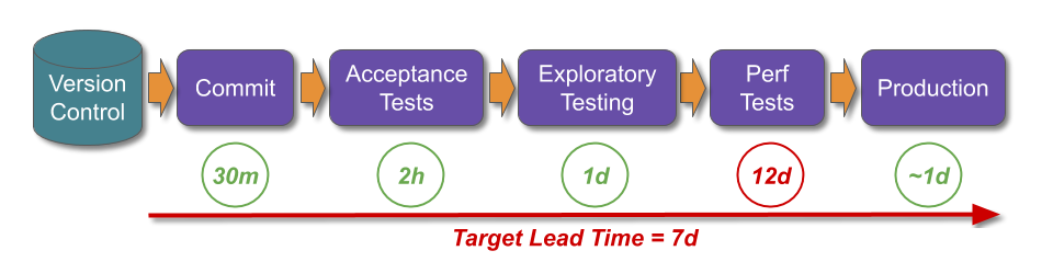
A short and wide deployment pipeline would also be unable to achieve the target lead time. The parallel testing activities would be limited by the 12 days of manual performance testing, and future release candidates would queue before the constrained activity. An obvious countermeasure would be for some release candidates to skip manual performance testing, but that would increase the risk of production incidents.

This means long and thin vs. short and wide deployment pipelines is a false dichotomy.

Pipeline Design and The Theory Of Constraints

In The Goal, Dr. Eli Goldratt describes the Theory Of Constraints as an iterative cycle known as the Five Focussing Steps: identify a constraint, reduce its wasted capacity, regulate its item arrival rate, increase its capacity, and then repeat.

If the activities in a technology value stream can be re-sequenced, re-designing a deployment pipeline is one way to reduce wasted time at a constrained activity, and regulate the arrival of release candidates. Pipeline flexibility is more important than any particular pipeline design, as it enables experimentation until a Goldilocks deployment pipeline can be found.

The constrained activity should not be the first activity after release candidate creation. This would reduce subsequent release candidate queues, and statistical fluctuations in unconstrained activities. However, constraint time should never be wasted on items with knowable defects, and most activities in a deployment pipeline are testing activities.

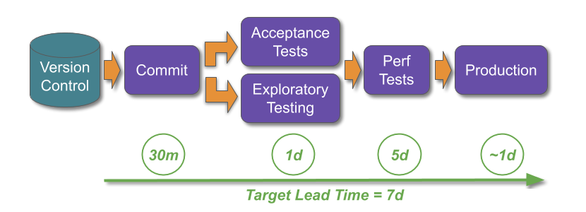
One Goldilocks deployment pipeline design is for all unconstrained testing activities to be parallelised before the constrained activity. This should be combined with other experiments to save constraint time, and regulate the flow of release candidates to minimise queues and statistical fluctuations. Such a pipeline design will make it easier for delivery teams to successfully implement Continuous Delivery.

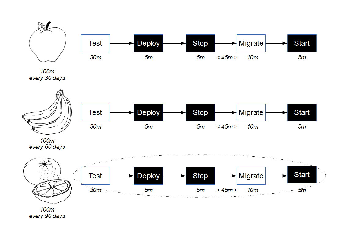
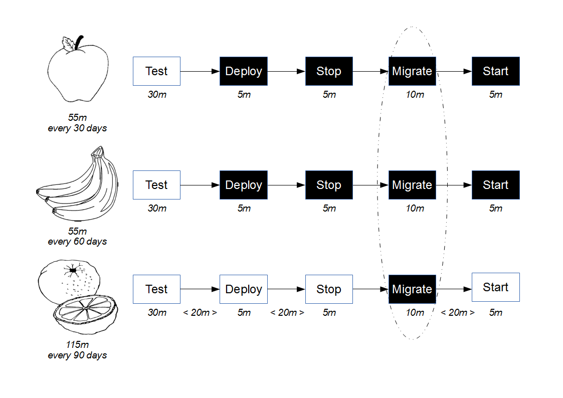
In the above example, assume the short and wide deployment pipeline can be re-designed so manual performance testing occurs after the other parallelised testing activities. This ensures release candidates with knowable defects are rejected prior to performance testing, which saves 1 day in queue time per release candidate. End-to-end performance testing scenarios are gradually replaced with stubbed performance tests and contract tests, which saves 6 days and means the target lead time can be accomplished. 

If there is no constrained activity in a technology value stream, the delivery team is in a state of Continuous Delivery and a constraint will exist either upstream in product development or downstream in customer marketing. Further deployment pipeline improvements such as automated filtering of test scenarios could increase the speed of release candidate feedback, but the priority should be tackling the external constraint if product cycle time from ideation to customer is to be improved.

Acknowledgements

Thanks to Thierry de Pauw for his feedback on this article.

Pipeline antipattern: Artifact Promotion

Promoting artifacts between repositories is a poor man’s metadata

Note: this antipattern used to be known as Mutable Binary Location

A Continuous Delivery pipeline is an automated representation of the value stream of an organisation, and rules are often codified in a pipeline to reflect the real-world journey of a product increment. This means artifact status as well as artifact content must be tracked as an artifact progresses towards production.

One way of implementing this requirement is to establish multiple artifact repositories, and promote artifacts through those repositories as they successfully pass different pipeline stages. As an artifact enters a new repository it becomes accessible to later stages of the pipeline and inaccessible to earlier stages.

For example, consider an organisation with a single QA environment and multiple repositories used to house in-progress artifacts. When an artifact is committed and undergoes automated testing it resides within the development repository.

Pipeline Antipattern Artifact Promotion - Development

When that artifact passes automated testing it is signed off for QA, which will trigger a move of that artifact from the development repository to the QA repository. It now becomes available for release into the QA environment.

Pipeline Antipattern Artifact Promotion - QA

When that artifact is pulled into the QA environment and successfully passes exploratory testing it is signed off for production by a tester. The artifact will be moved from the QA repository to the production repository, enabling a production release at a later date.

Pipeline Antipattern Artifact Promotion - Production

A variant of this strategy is for multiple artifact repositories to be managed by a single repository manager, such as Artifactory or Nexus.

Pipeline Antipattern Artifact Promotion - Repository Manager

This strategy fulfils the basic need of restricting which artifacts can be pulled into pre-production and production environments, but its reliance upon repository tooling to represent artifact status introduces a number of problems:

  • Reduced feedback – an unknown artifact can only be reported as not found, yet it could be an invalid version, an artifact in an earlier stage, or a failed artifact
  • Orchestrator complexity – the pipeline runner has to manage multiple repositories, knowing which repository to use for which environment
  • Inflexible architecture – if an environment is added to or removed from the value stream the toolchain will have to change
  • Lack of metrics – pipeline activity data is limited to vendor-specific repository data, making it difficult to track wait times and cycle times

A more flexible approach better aligned with Continuous Delivery is to establish artifact status as a first-class concept in the pipeline and introduce per-binary metadata support.

Pipeline Antipattern Artifact Promotion - Metadata

When a single repository is used, all artifacts reside in the same location alongside their versioned metadata, which provides a definitive record of artifact activity throughout the pipeline. This means unknown artifacts can easily be identified, the complexity of the pipeline orchestrator can be reduced, and any value stream design can be supported over time with no changes to the repository itself.

Furthermore, as the collection of artifact metadata stored in the repository indicates which artifact passed/failed which environment at any given point in time, it becomes trivial to pipeline dashboards that can display pending releases, application cycle times, and where delays are occurring in the value stream. This is a crucial enabler of organisational change for Continuous Delivery, as it indicates where bottlenecks are occurring in the value stream – likely between people working in separate teams in separate silos.

Pipeline pattern: Analysis Stage

Separate out analysis to preserve commit stage processing time

The entry point of a Continuous Delivery pipeline is its Commit Stage, and as such manages the compilation, unit testing, analysis, and packaging of source code whenever a change is committed to version control. As the commit stage is responsible for identifying defective code it represents a vital feedback loop for developers, and for that reason Dave Farley and Jez Humble recommend a commit stage that is “ideally less than five minutes and no more than ten” – if the build process is too slow or non-deterministic, the pace of development can soon grind to a halt.

Both compilation and unit testing tasks can be optimised for performance, particularly when the commit stage is hosted on a multi-processor Continuous Integration server. Modern compilers require only a few seconds for compilation, and a unit test suite that follows the Michael Feathers strategy of no database/filesystem/network/user interface access should run in parallel in seconds. However, it is more difficult to optimise analysis tasks as they tend to involve third-party tooling reliant upon byte code manipulation.

When a significant percentage of commit stage time is consumed by static analysis tooling, it may become necessary to trade-off unit test feedback against static analysis feedback and move the static analysis tooling into a separate Analysis Stage. The analysis stage is triggered by a successful run of the commit stage, and analyses the uploaded artifact(s) and source code in parallel to the acceptance testing stage. If a failure is detected the relevant pipeline metadata is updated and Stop The Line applies. That artifact cannot be used elsewhere in the pipeline and further development efforts should cease until the issue is resolved.

For example, consider an organisation that has implemented a standard Continuous Delivery pipeline. The commit stage has an average processing time of 5 minutes, of which 1 minute is spent upon static analysis.

Over time the codebase grows to the extent that commit stage time increases to 6 minutes, of which 1 minute 30 seconds is spent upon static analysis. With static analysis time growing from 20% to 25% the decision is made to create a separate Analysis stage, which reduces commit time to 4 minutes 30 seconds and improves the developer feedback loop.

Static analysis is the definitive example of an automated task that periodically needs human intervention. Regardless of tool choice there will always be a percentage of false positives and false negatives, and therefore a pipeline that implements an Analysis Stage must also offer a capability for an authenticated human user to override prior results for one or more application versions.

Continuous Delivery and Cost of Delay

Use Cost of Delay to value Continuous Delivery features

When building a Continuous Delivery pipeline, we want to value and prioritise our backlog of planned features to maximise our return on investment. The time-honoured, ineffective IT approach of valuation by intuition and prioritisation by cost is particularly ill-suited to Continuous Delivery, due to its focus upon one-off infrastructure improvements to enable product flow. How can we value and prioritise our backlog of planned pipeline features to maximise economic benefits?

To value our backlog, we can calculate the Cost of Delay of each feature – its economic value over a period of time if it was immediately available. Described by Don Reinertsen as “the golden key that unlocks many doors“, Cost of Delay can be calculated by quantifying the value of change or the cost of the status quo via the following economic benefit types:

  • Increase Revenue – improve profit margin
  • Protect Revenue – sustain profit margin
  • Reduce Costs – reduce costs currently incurred
  • Avoid Costs – reduce costs potentially incurred

Cost of Delay allows us to quantify the opportunity cost between a feature being available now or later, and using money as the unit of measurement transforms stakeholder conversations from cost-cutting to delivering value. Calculation accuracy is less important than the process of collaborative information discovery, with assumptions and probabilities preferably co-owned by stakeholders and published via information radiator.

Cost of Delay = economic value over time if immediately available

To prioritise our backlog, we can use Cost of Delay Divided By Duration (CD3) – a variant of the Weighted Shortest Job First scheduling policy. With CD3 we divide Cost of Delay by duration, with a higher score resulting in a higher priority. This is an effective scheduling policy as the duration denominator promotes batch size reduction.

CD3 = Cost of Delay / Duration

As the goal of Continuous Delivery is to decrease cycle time by reducing the transaction cost of releasing software, a pipeline feature will likely yield an Avoid Cost or Reduce Cost benefit intrinsically linked to release cadence. We can therefore calculate the Cost of Delay as one of the below:

  1. Reduce Cost: Automate action(s) to decrease wait times within release processing time

    = (wait time in minutes / cycle time in days) * minute price in £

  2. Avoid Cost: Automate action(s) to decrease probability of repeating release processing time due to rework

    = (processing time in minutes / cycle time in days) * minute price in £ * % cost probability per year

For example, consider an organisation building a Continuous Delivery pipeline to support its Apples, Bananas, and Oranges applications by fully automating its release scripts. The rate of business change is variable, with an Apples cycle time of 1 month, a Bananas cycle time of 2 months, and an Oranges cycle time of 3 months. Our pipeline has already fully automated the deploy, stop, and start actions for our Apples and Bananas applications but lacks support for our Oranges application, our test framework, and our database migrator.
Application Estate Once our development team have provided their cost estimates, how do we determine which feature to implement next without resorting to intuition?

Backlog Duration We begin by agreeing with our pipeline stakeholders an arbitrary price for a minute of our time of £10000, and calculate the Cost of Delay for supporting the Oranges application as:
Support Oranges application

= (wait time / cycle time) * minute price
= (20 + 20 + 20 / 90) * 10000
= 0.67 * 10000
= £6700 per day

Given the test framework has failed twice in the past year and caused a repeat of release processing time specifically due to its lack of pipeline support, the Cost of Delay is:
Support test framework

= (100 / months in a year) * occurrences
= (100 / 12) * 2
= 16% cost probability per year

= (processing time / cycle time) * minute price * % cost probability
= ((100 / 30) + (100 / 60) + (160 / 90)) * 10000 * 16%
= 6.78 * 10000 * 16%
= £10848 per day (£5328 Apples, £2672 Bananas, £2848 Oranges)

The Cost of Delay for supporting the database migrator is:

Support database migrator

= (wait time / cycle time) * minute price
= ((45 / 30) + (45 / 60) + (45 / 90)) * 10000
= 2.75 * 10000
= £27500 per day (£15000 Apples, £7500 Bananas, £5000 Oranges)

Now that we have established the value of the planned pipeline features, we can use CD3 to produce an optimal work queue. CD3 confirms that support for the database migrator is our most urgent priority:

Backlog CD3

This example shows that using Cost of Delay and CD3 within Continuous Delivery validates Mary Poppendieck’s argument that “basing development decisions on economic models helps the development team make good tradeoff decisions“. As well as learning support for the database migrator is twice as valuable as any current alternative, we can offer new options to our pipeline stakeholders – for example, if an Apples-specific database migrator required only 5 days, it would become our most desirable feature (£15000 per day / 5 days = CD3 score of 3000).

Updating a Pipeline

Pipeline updates must minimise risk to protect the Repeatable Reliable Process

We want to quickly deliver new features to users, and in Continuous Delivery Dave Farley and Jez Humble showed that “to achieve these goals – low cycle time and high quality – we need to make frequent, automated releases“. The pipeline constructed to deliver those releases should be no different and frequently, automatically released into Production itself. However, this conflicts with the Continuous Delivery principle of Repeatable Reliable Process – a single application release mechanism for all environments, used thousands of times to minimise errors and build confidence – leading us to ask:

Is the Repeatable Reliable Process principle endangered if a new pipeline version is released?

To answer this question, we can use a risk impact/probability graph to assess if an update will significantly increase the risk of a pipeline operation becoming less repeatable and/or reliable.

Pipeline Risk

This leads to the following assessment:

  1. An update is unlikely to increase the impact of an operation failing to be repeatable and/or reliable, as the cost of failure is permanently high due to pipeline responsibilities
  2. An update is unlikely to increase the probability of an operation failing to be repeatable, unless the Published Interface at the pipeline entry point is modified. In that situation, the button push becomes more likely to fail, but not more costly
  3. An update is likely to increase the probability of an operation failing to be reliable. This is where stakeholders understandably become more risk averse, searching for a suitable release window and/or pinning a particular pipeline version to a specific artifact version throughout its value stream. These measures may reduce risk for a specific artifact, but do not reduce the probability of failure in the general case

Based on the above, we can now answer our original question as follows:

A pipeline update may endanger the Repeatable Reliable Process principle, and is more likely to impact reliability than repeatability

We can minimise the increased risk of a pipeline update by using the following techniques:

  • Change inspection. If change sets can be shown to be benign with zero impact upon specific artifacts and/or environments, then a new pipeline version is less likely to increase risk aversion
  • Artifact backwards compatibility. If the pipeline uses a Artifact Interface and knows nothing of artifact composition, then a new pipeline version is less likely to break application compatibility
  • Configuration static analysis. If each defect has its root cause captured in a static analysis test, then a new pipeline version is less likely to cause a failure
  • Increased release cadence. If the frequency of pipeline releases is increased, then a new pipeline version is more likely to possess shallow defects, smaller feedback loops, and cheaper rollback

Finally, it is important to note that a frequently-changing pipeline version may be a symptom of over-centralisation. A pipeline should not possess responsibility without authority and should devolve environment configuration, application configuration, etc. to separate, independently versioned entities.

Pipeline Antipattern: Uber-Artifact

Pipelining inter-dependent applications as uber-artifacts is unscalable

Achieving the Continuous Delivery of an application is a notable feat in any organisation, but how do we build on such success and pipeline more complex, inter-dependent applications? In Continuous Delivery, Dave Farley and Jez Humble suggest an Integration Pipeline architecture as follows:

Integration Pipeline

In an Integration Pipeline, the successful commit of a set of related application artifacts triggers their packaging as a single releasable artifact. That artifact then undergoes the normal test-release cycle, with an increased focus upon fast feedback and visibility of binary status.

Although Eric Minick’s assertion that this approach is “broken for complex architectures” seems overly harsh, it is true that its success is predicated upon the quality of the tooling, specifically the packaging implementation.

For example, a common approach is the Uber-Artifact (also known as Build Of Builds or Mega Build), where an archive is created containing the application artifacts and a version manifest. This suffers from a number of problems:

  • Inconsistent release mechanism. The binary deploy process (copy) differs from the uber-binary deploy process (copy and unzip)
  • Duplicated artifact persistence. Committing an uber-artifact to theartifact repository re-commits the constituent artifacts within the archive
  • Lack of version visibility. The version manifest must be extracted from the uber-artifact to determine constituent versions
  • Non-incremental release mechanism. An uber-artifact cannot easily diff constituent versions and must be fully extracted to the target environment

Of the above, the most serious problem is the barrier to incremental releases, as it directly impairs pipeline scalability. As the application estate grows over time in size and/or complexity, an inability to identify and skip the re-release of unchanged application artifacts can only increase cycle time.

Returning to the intent of the Integration Pipeline architecture, we simply require a package that expresses the relationship between the related application artifacts. In an uber-artifact, the value resides in the version manifest – so why not make that the artifact?

The Merit of Metadata

Metadata increases feedback and ensures value stream integrity

In Continuous Delivery, Dave Farley and Jez Humble describe the Lean production principles that underpin Continuous Delivery, and how a pipeline encapsulates a value stream – the journey a customer feature undertakes from discovery to real world consumption.

In a pipeline each stage represents a step in the value stream, meaning that for application XYZ an example value stream of [Development -> Acceptance -> UAT -> Performance -> Production] could be defined as follows:

Pipeline with Metadata

In the above pipeline, each stage ends with a discrete piece of metadata (“created XYZ 2.1”, “XYZ 2.1 passed acceptance tests”, etc.) being written back to the binary repository, indicating that one or more new customer features have progressed in the value stream.

Unfortunately, pipelines are often constructed without metadata support:

Pipeline without Metadata

In this situation the lack of activity data reduces each stage to a fire-and-forget operation, constraining feedback and unnecessarily exposing the value stream to obtuse, time-consuming errors. For example, QA could mistakenly test new features that have not passed automated regression tests, or Operations could mistakenly release features that have not been signed off.

With metadata the following safeguards can be easily implemented:

  • Check if binary actually exists e.g. “can XYZ 1.2 be retrieved for deploy to Production”
  • Prevent binary re-entering a previous stage e.g. “once XYZ 1.2 has passed or failed Acceptance, the result is final”
  • Ensure binary has successfully passed sufficient dependencies to enter a stage e.g. “XYZ 1.2 can only enter Production once it has successfully passed UAT and Performance”
  • Introduce a manual sign-off process for critical environments e.g. “XYZ 1.2 can only pass UAT when exploratory testing is complete”
  • Visualise pipeline activity e.g. “I can see XYZ 1.2 was successfully released to Production a week ago, and that 1.4 is the next viable candidate as 1.3 failed Acceptance”

These features ensure fast feedback is always available and that the pipeline is an accurate representation of the underlying value stream. An absence of metadata unnecessarily hinders these goals and suggests a failure to understand the core values of Continuous Delivery.

Pipeline Antipattern: Deficient Deployer

A badly-defined Deployer abstraction impairs Continuous Delivery

As Continuous Delivery patterns are gradually establishing themselves, antipatterns are also surfacing – and a common antipattern is the Deficient Deployer.

When we talk about a Deployer, we are referring to a pipeline task that can be invoked by any post-Commit stage to deliver an application binary to an environment. A Deployer interface should look like:

Deployer#Deploy(Application a, Version v, Environment e)

There are a couple of ways Deficient Deployer can creep into a Deployer implementation:

  • Anemic implementation – this is where the Deployer behaviour is solely specified as “download binary and copy to environment”, ignoring any one-time operations deemed necessary for a binary to be in a valid state. For example, environment configuration should be filtered into the application binary during deployment, as it is a one-time operation decoupled from the application lifecycle. If this configuration step is omitted from the Deployer, then additional manual effort(s) will be required to make the binary ready for use.
  • Over-specified interface – this is where environment-specific parameters are added to the Deployer interface e.g. Deployer#Deploy(Application a, Version v, Environment e, Server s). The server(s) associated with an environment and their credentials should be treated as an implementation detail of the Deployer via a per-environment server mapping. Application version, and environment are the only consistent mandatory parameters across all environments.

The root cause of the Deficient Deployer seems to be a reluctance to treat deployment scripts as first class citizens.

© 2024 Steve Smith

Theme by Anders NorénUp ↑