How should you actually implement Continuous Delivery?
Adopting Continuous Delivery takes time. You have a long list of technology and organisational changes to consider. You have to work within the unique circumstances of your organisation. You’re constantly surrounded by strange problems, half-baked theories, off the shelf solutions that just don’t work, and people telling you Amazon is nothing to worry about
How do you identify and remove the major impediments in your build, testing, and operational activities? How do you avoid spending weeks, months, or years on far-reaching changes that ultimately have no impact on your time to market?
TL;DR:
- Continuous Delivery means applying technology and organisational changes to the unique circumstances of an organisation
- If a Continuous Delivery programme does not focus on the activities with the most rework and/or queue times, there is a high probability of sub-optimal outcomes
- The Theory Of Constraints is a management paradigm for improving organisational throughput, while simultaneously decreasing both inventory and operating expense.
- The Theory Of Constraints can be applied to Continuous Delivery, as the build, testing, and operational activities in a technology value stream should be homogeneous
- The Five Focussing Steps can be used to identify constrained activities, and then introduce the necessary technology and organisational changes to reduce rework and/or queue times
Introduction
Technology can bring benefits if, and only if, it diminishes a limitation – Dr. Eli Goldratt
An organisation will have one or more technology value streams. Each one will represent a sequence of activities that converts business ideas into value-adding software for customers. The first part of a technology value stream will be design and development activities, which are inherently non-deterministic and highly variable. The second part will be build, testing, and operational activities, which should be as deterministic and invariable as possible. When an organisation lacks the necessary stability and throughput in its technology value streams to satisfy market demand, it is in a state of Discontinuous Delivery.
Continuous Delivery is a set of holistic principles and practices to improve the stability and throughput of IT delivery. It needs a substantial investment in technology changes:
- Version Control: put code, configuration, infrastructure definitions, migration scripts, etc. in version control to preserve change history
- Environments: automate self-service, on-demand provisioning of short-lived test environments and incremental release patterns such as Canary Deployments
- Development: use Test Driven Development with Pair-Programming to build quality into a codebase, and use Trunk Based Development with Continuous Integration to ensure it is always releasable
- Architecture: establish an Evolutionary Architecture to encourage loosely-coupled, independently deployable services
- Testing: automate parallelisable acceptance tests with dynamic test data, use Smoke Testing to validate deployments, and use Exploratory Testing to uncover new information
- Operability: aggregate logs and metrics to create a centralised telemetry platform for visualising normal conditions, and alerting on abnormal conditions
It also requires a significant amount of organisational changes:
- Batch Size: reduce features per release candidate to decrease variability, feedback delays, risk, overheads, inefficiencies, and lead time via Little’s Law
- Management: devolve decision making to the employees closest to the work to empower better choices in design, testing etc.
- Culture: grow a performance-oriented culture of cooperation and collaboration to increase information flow between teams
- Responsibilities: change responsibilities for testing and on-call production support to encourage a shared sense of accountability
- Risk: use continuous code reviews via Pair-Programming and traceability of production changes to replace Risk Management Theatre with adaptive risk assessment
- Skills: invest in employee training to ease the introduction of new practices and tools e.g. infrastructure automation
- Structures: convert siloed functional teams into cross-functional teams, and align team and software architecture with Conway’s Law to enable faster delivery
These changes are challenging in isolation, but it is their application to the unique circumstances and constraints of an organisation that makes Continuous Delivery so difficult. Adopting Continuous Delivery means implementing widespread changes in the highly uncertain conditions of a complex, adaptive system, in which behaviours are emergent and interactions are unpredictable.
A Continuous Delivery programme should aim to reduce rework and queue times in a technology value stream, as they are the most common sources of waste. Rework is any activity that must be repeated due to a failure, such as a tester being given a defective release candidate. Queue time is time spent queuing for an activity, such as a deployment waiting for a tester to become available. There are many potential causes of rework and queue time, including the following:
| Cause | Description |
|---|---|
| Snowflake environments | Manual environment provisioning |
| Brittle deployments | Unreliable code, config, or infra changes |
| Environment contention | Slow access to test data, services, or environments |
| End-To-End Testing | Reams of slow, non-deterministic tests |
| Rigid architecture | Application deployments coupled together |
| Excessive toil | Manual, repetitive build/testing/operations tasks |
Over the years, the advice on how to implement Continuous Delivery has evolved. The Continuous Delivery book suggested using the Plan-Do-Check-Act Cycle to experiment with changes, and implement a maturity model. Lean Enterprise recommended the Improvement Kata be used to create a Continuous Improvement framework, with Plan-Do-Check-Act used to structure different experiments. This can be very effective, but there needs to be a way to focus on the activities where a reduction in rework and/or queue times will have an immediate, positive impact. Otherwise, there is a high probability of sub-optimal outcomes, stakeholder dissatisfaction, and Discontinuous Delivery remaining the norm.
Given sufficient Continuous Delivery expertise, heuristics can be used to locate those activities in a technology tech value stream. An alternative method is needed when those heuristics are unavailable, or insufficient to overcome resistance to change.
Example – Network Activation
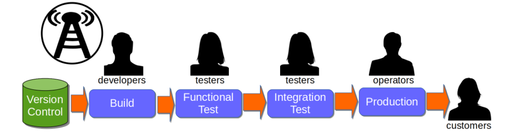
Think of an 18 month Continuous Delivery programme for a multi-team, multi-application Network Activation platform. The delivery teams already use Pair-Programming, Test-Driven Development, Trunk Based Development, and Continuous Integration. The on-prem technology value stream has 2 pre-production activities – Functional Test and Integration Test – and a production deployment involves 10 semi-automated and manual tasks. Problems include snowflake environments, brittle deployments, and End-To-End Testing. There is no data on deployments, beyond an average lead time to production of 34 days. The product owner wants it to be 14 days.
Over 18 months there is a concerted effort to create a consistent deployment pipeline, with the Cost of Delay used to prioritise pipeline features. Aggregate Artifacts and Artifact Containers are used to automate deployments, infrastructure provisioning errors are eliminated, and pipeline dashboards are built. Verify Branch By Abstraction is used to incrementally decouple applications, by replacing object serialisation with RESTful APIs. API Examples and Consumer Driven Contracts are used to verify application interactions. There are also a series of organisational changes to policies, processes, and teams, to reduce queue time for Functional Test and Integration Test.
These changes produce many benefits, including a 95% build time improvement from 1 hour to 3 minutes, and a 43% improvement in test deployment time from 3.5 hours to 2.5 hours. However, there is no impact whatsoever on the average lead time of 34 days. On that basis, the Continuous Delivery programme is unsuccessful.
The Theory Of Constraints
In The Goal, Dr. Eli Goldratt sets out the Theory Of Constraints. The Theory Of Constraints is a management paradigm for improving organisational throughput, by optimising a small number of constraints in a homogeneous workflow. It states the goal of an organisation is to make money, by increasing throughput while simultaneously decreasing both inventory and operating expense.
A constraint is any resource with capacity equal to or less than market demand, and it will limit the throughput of the organisation. A constraint is internal when market demand is greater than throughput, and external when throughput is greater than market demand. An hour lost at a constraint is an hour lost for the whole organisation.
A non-constraint is any resource with capacity greater than market demand. The level of utilisation of a non-constraint is determined by a constraint elsewhere. An increase in non-constraint capacity is a waste of time and money, as it can only increase queued work before a constraint and cannot reduce work starvation after a constraint. An hour lost at a non-constraint is an illusion.
The central premise of the Theory Of Constraints is to iteratively increase the capacity of a constraint, until the flow of work items can be balanced according to market demand. The Five Focussing Steps are used to achieve this:
- Identify the constraint(s): calculate market demand for a product, and which activities have capacity less than or equal to demand
- Exploit the constraint(s): increase constraint utilisation by eliminating idle time, and time wasted on lower priority and/or defective work items
- Subordinate everything else to the constraint(s): protect a constraint from excessive inventory or work starvation by maintaining a buffer of materials, and regulating the arrival of new work items into the system based on constraint capacity
- Elevate the constraint(s): offload constraint work items to a non-constraint by investing in additional equipment, people, and/or allocation of work items to third parties
- If a constraint has been broken, go back to step 1, but do not allow inertia to cause a constraint
Continuous Delivery and the Theory Of Constraints
The Theory Of Constraints can be applied to Continuous Delivery, as the build, testing, and operations activities in a technology value stream should be homogeneous. There will be one, or at most a few constrained activities, caused by rework and/or queue times. The Five Focussing Steps can be used to identify and optimise the constraint(s), until the flow of release candidates is balanced from mainline commit to production and Continuous Delivery is achieved. At that point, an external constraint will emerge upstream in product development or downstream in sales. If market demand increases later on, a new internal constraint might surface within the technology value stream.
Identify the constraint
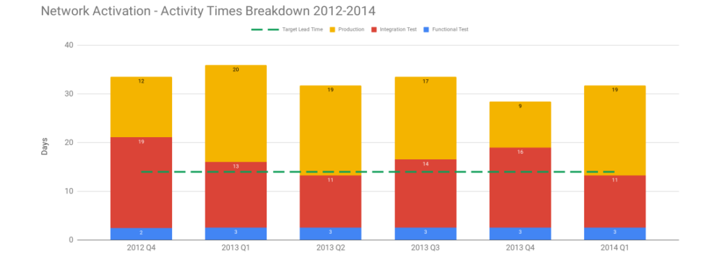
A constraint is identified by establishing the market demand for a product, and then calculating how much time each activity contributes to meeting that demand. Overall market demand should be specified by the product owner as a target Lead Time lt, and measured from mainline commit to production launch.
lt = X minutes/hours/days
The ability of an activity a n to meet lt should be expressed as its Activity Time at n. It can be measured as the median between its finish time aft n and the finish time of the prior activity aft n – 1, for all occurrences of a n in a time period t. This measurement ensures queue time and process time are both accounted for. The measurement unit should be minutes, hours, or days based on lt. It might be necessary to measure variability in Activity Time as well, if one or more activities exhibit an undesirable amount of variability.
at n = median ( ( aft n - aft n - 1 ) for a n in t )
If an activity has at n greater than lt, it is a constraint. If a high percentage of release candidates consistently fail to pass the activity on the first attempt, it is unstable and rework must be reduced. Alternatively, if release candidates are regularly delayed before starting the activity, it is too slow to begin and queue time must be reduced.
If no activity has at n greater than lt, there is no internal constraint. This means lt is not ambitious enough, or there is an external constraint outside the technology value stream.
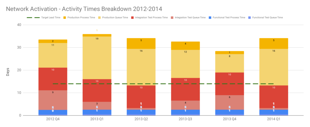
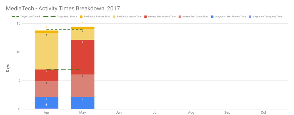
Applying the Theory Of Constraints to the Network Activation platform with its target lead time of 14 days reveals a constraint. Visualising each activity as queue time and process time shows Production queue time was often greater than 14 days. This was caused by a well-intentioned release management policy of deploying release candidates into production when ready, and then waiting for a launch date pre-agreed with an upstream billing provider months earlier. Launch dates were delayed when testing finished late, but never brought forward when testing finished early. 18 months of hard work reduced variability, Functional Test queue time, and Integration Test queue time, but those improvements merely led to an increase in Production queue time until launch dates occurred.
Optimise the constraint
A constraint is optimised by experimenting with the full range of technology and organisational changes recommended by Continuous Delivery. There needs to be a concerted effort to reduce the average and variation in Activity Time for the constrained activity, until the target Lead Time can be satisfied.
Exploiting a constrained activity means ensuring it is always working, and always doing valuable work. This aligns with Continuous Delivery emphasising the automation of repetitive tasks to free up people for higher-order problems. Automated infrastructure provisioning, automated unit and acceptance testing, and moving to an Evolutionary Architecture are all examples of technology changes to reduce time spent at a constrained activity. The most effective organisational change is to reduce batch sizes, as a smaller batch will have shorter process times and queue times.
Subordinating unconstrained activities means limiting the flow of mainline commits, builds, and deployments to match the constrained activity. This is best accomplished with Work In Process (WIP) Limits, which encourage people to collaborate on a few work items at any point in time. Stop The Line teaches people to prioritise a releasable codebase over developing more features, and eXtreme Programming practices such as Test-Driven Development and Pair-Programming can also foster a shared team cadence.
Elevating a constrained activity means investing in people and tools to increase its capacity. This might be achieved with technology changes, such as a move to short-lived test environments via fully automated infrastructure provisioning. It might also involve organisational changes such as paying third party suppliers for more test data, hiring more engineers, or running training courses to improve Staff Liquidity.
For instance, an assortment of changes should be tried if End-To-End Testing activity is a constraint. Time wasted should be eliminated by ensuring testers are uninterruptible, making more testers available, and running testing slots 24 hours a day. Defective release candidates should be minimised by moving all other testing activities in front of End-To-End Testing, adding automated contract tests, and rejecting release candidates with one or more test failures. Over time the end-to-end tests should be incrementally replaced with automated acceptance tests, monitoring dashboards, and automated anomaly detection.
Example: MediaTech
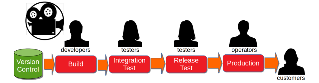
Consider a 7 month Continuous Delivery programme for a multi-team, multi-application MediaTech platform. The delivery teams use Trunk Based Development with some Pair Programming, but there is little Test-Driven Development. The on-prem technology value stream has 2 pre-production activities – Functional Test and Release Test – and a production deployment involves 60 semi-automated and manual tasks. Problems include snowflake environments, brittle deployments, environment contention, a rigid architecture, End-To-End Testing, and excessive toil. There is no data on deployments, beyond an average interval of 3 weeks. The product owner has set a target lead time of 1 week, at an interval of 1 week.
The range of problems at MediaTech makes Continuous Delivery very challenging. There is a proposal to create a fully automated deployment pipeline, with infrastructure provisioning, deployments, and telemetry. Other suggested options include the promotion of Test-Driven Development, implementing zero downtime deployments, and immutable release candidates. However, there are concerns about the time needed to make such changes.
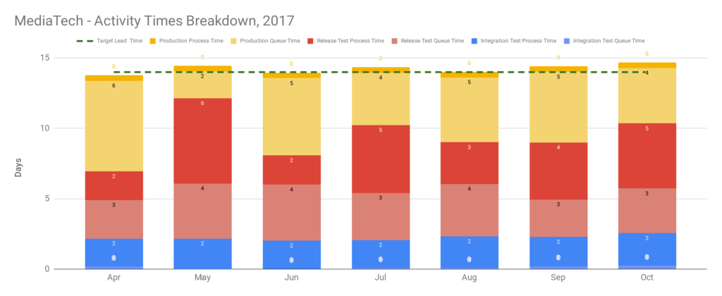
After 2 months, deployment data is scraped from chat channels, and applying the Five Focussing Steps shows sweeping changes are not immediately required. The constraint on a target lead time of 1 week is Release Test process time, due to perennial environment instability caused by configuration and test data issues. Interestingly, there is no obvious constraint on a target lead time of 2 weeks. As a result, the product owner agrees to a target lead time of 2 weeks at an interval of 2 weeks, as an intermediate milestone.
In the Theory Of Constraints, a lack of skilled people can constitute a constraint. When the above data is shared with the MediaTech operations team, they reveal an unseen constraint on the 14 day target lead time. There is a single release planner, who endures a heavy workload for each production deployment on top of their day to day work. Everyone agrees the Continuous Delivery programme needs to focus on automating the release planning tasks, and improving the existing automated tests.
Over the next few months, the release planning workload is reduced and the automated tests are stabilised. Callout rota emails by the release planner are replaced by a shared rota, co-owned by the delivery teams. A release note process overseen by the release planner involving 3 different teams is replaced by a fully automated release note tool. Furthermore, end-to-end tests in Integration Test and Release Test are prioritised by their non-determinism, and gradually rewritten as build-time acceptance tests. The target lead time of 2 weeks at an interval of 2 weeks is successfully achieved, and after several production deployments the product owner decides the new throughput is sufficient. The Continuous Delivery programme is considered a success, and without a fully automated deployment pipeline.
Further Reading
- Beyond The Goal by Dr. Eli Goldratt
- Measuring Continuous Delivery by the author
- Resilience as a Continuous Delivery Enabler by the author
Acknowledgements
Thanks to Thierry de Pauw for his feedback on this article.
![Economic Batch Size [Reinertsen]](https://www.stevesmith.tech/wp-content/uploads/2013/03/Economic-Batch-Size-Reinertsen.jpg)
Recent Comments