Continuous Delivery reduces defect probability and cost
Continuous Delivery often challenges conventional wisdom within the IT industry, and by advocating the rapid release of value-add to reduce risk it contradicts the traditional belief that a low release cadence is an effective risk reduction strategy. How can releasing software more frequently reduce both defect probability and defect cost?
The probability of a defect is the likelihood of a change within a changeset unexpectedly impeding value-add and imposing an opportunity cost. Given the defect probability of a changeset is proportional to its size we can calculate the defect probability of a change as follows:
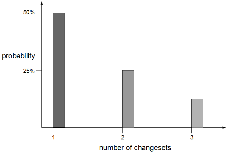
n = number of changesets
probability = (1 / 2n) * 100 [percentage]
The above formula indicates that decreasing changeset size by increasing the number of changesets will reduce defect probability, and this is confirmed by Don Reinertsen’s assertion that “many smaller experiments produce less variation than one big one“. For example, if a change is released in 1 changeset there is a 1 in 2 chance or 50% probability of failure. If it was instead released in 3 changesets there would be a 1 in 8 chance or 12.5% probability of failure.
The cost of a defect is the product of cost per unit time and duration, where cost per unit time represents economic impact and duration represents lifetime.
cost = cost per unit time [currency] * duration [unit time]
A defect has an inception date at its outset, a discovery date when diagnosed, and a resolution date when fixed. The interactions between these dates and cost per unit time enable a division of defect cost into sunk cost and opportunity cost. The sunk cost of a defect represents the economic damage already incurred at the point of discovery, while opportunity cost represents the economic damage still to be incurred.
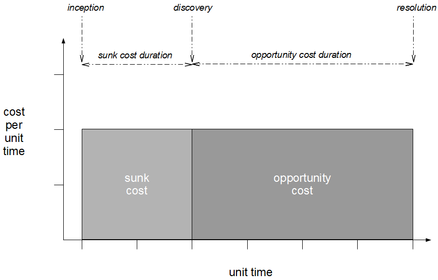
sunk cost duration = discovery date – inception date [unit time]
sunk cost = cost per unit time * sunk cost duration [currency]opportunity cost duration = resolution date – discovery date [unit time]
opportunity cost = cost per unit time * opportunity cost duration [currency]cost = sunk cost + opportunity cost [currency]
As cost per unit time is controlled by market conditions it is far easier to reduce opportunity cost duration by shortening lead times. This can be accomplished via batch size reduction, as Mary and Tom Poppendieck have observed that “time through the system is directly proportional to the amount of work-in-process” due to Little’s Law:
lead time = work in progress [units] / completion rate [units per time period]
Little’s Law is universal for all stable systems in which these variables are consistent long-term averages, and it is mathematical proof that reducing batch size will reduce lead time. For example, if a jug contains 4 litres of water and pours 2 litres per second then it will empty in 2 seconds. If instead the jug contained 2 litres of water and still poured 2 litres per second it would empty in 1 second.
Releasing smaller changesets more frequently into production can also reduce sunk cost duration, as small batches accelerate feedback. A smaller batch size will decrease the lead time and complexity associated with each changeset, creating faster feedback loops that will reduce the time required to discover a defect.
Consider an organisation with an average changeset size of 24 changes and an average lead time of 12 days. How can we reduce the defect probability of the next production release R1?
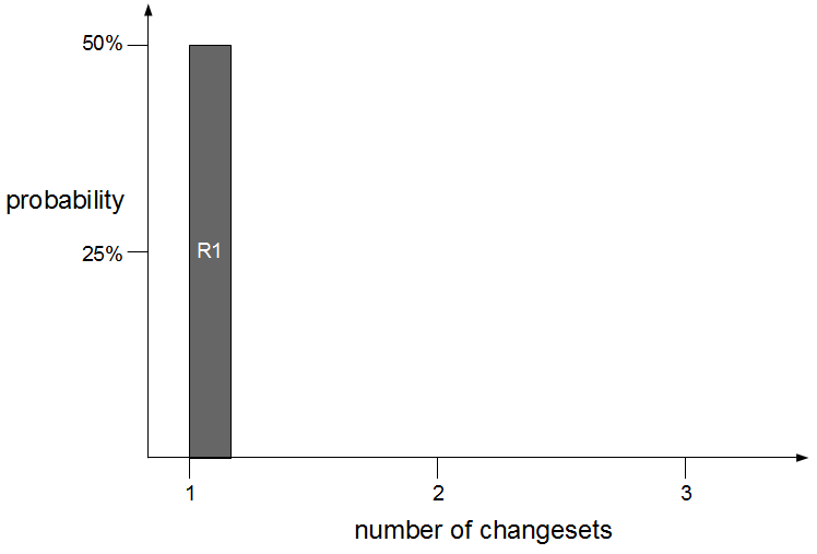
n = 1
probability = (1 / 21) * 100 = 50%
Based on the binomial probabilities involved we recommend to the organisation that it reduce defect probability by applying batch size reduction to R1 and splitting its changeset into 2 smaller releases R1 and R2. This would decrease defect probability from 50% to 25%.
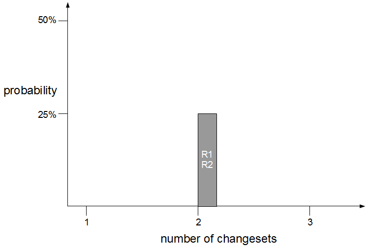
n = 2
probability = (1 / 22) * 100 = 25%
Unfortunately the organisation ignores our advice to release smaller changesets, and the release of R1 at a later date introduces a defect D1 that remains undiscovered for 6 days. D1 impedes a sufficient amount of value-add that a cost per unit time of £20,000 per day is estimated, which means a sunk cost of £120,000 has already been incurred and an opportunity cost of £240,000 is forecast. The organisation immediately triages D1 for a fix, but how can we reduce its opportunity cost?
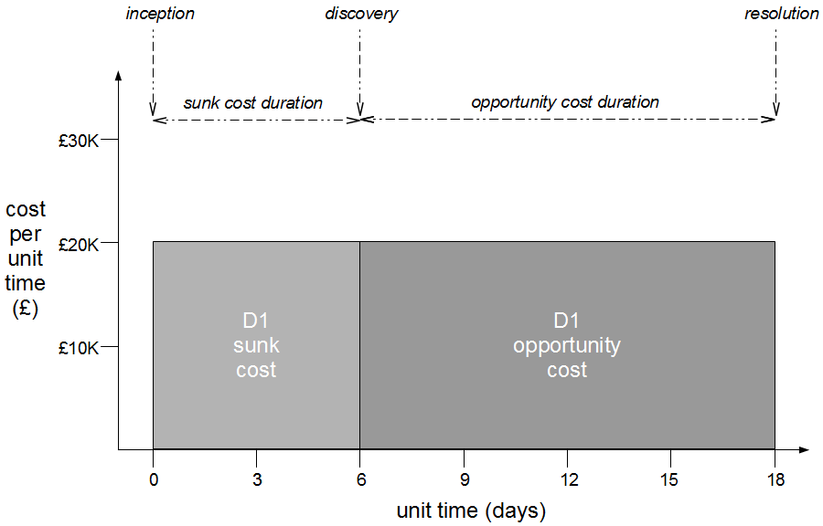
cost per unit time = £20,000
sunk cost = 6 days * £20,000 = £120,000
opportunity cost = 12 days * £20,000 = £240,000
overall cost = sunk cost + opportunity cost = £360,000
Given the organisation currently has an average batch size of 24 changes per changeset and a 12 day average lead time, Little’s Law computes an average completion rate of 2 changes per day and informs us that a reduced batch size of 12 changes per changeset would produce a 6 day lead time.
completion rate = work in process / lead time
completion rate = 24 changes per changeset / 12 days = 2 changes per daylead time = work in process / completion rate
lead time = 12 changes per changeset / 2 changes per day = 6 days
Based on Little’s Law we again recommend to the organisation a halved batch size of 12 changes per changeset, and this time our advice is accepted. A fix for D1 is included in the next changeset released into production in 6 days, which produces an opportunity cost saving of £120,000.
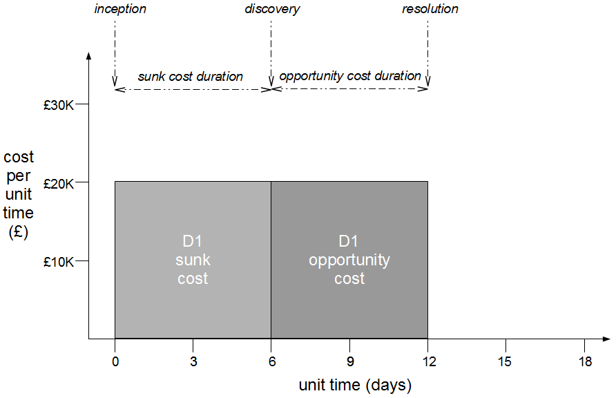
cost per unit time = £20,000
sunk cost = 6 days * £20,000 = £120,000
opportunity cost = 6 days * £20,000 = £120,000
overall cost = sunk cost + opportunity cost = £240,000
As well as decreasing the total cost of D1 by 33%, the new lead time of 6 days increases the rate of feedback for future production defects. When a subsequent release introduces defect D2 at a lower cost per unit time of £10,000 per day the reduced size and complexity of the offending changeset means D2 is discovered in only 3 days.
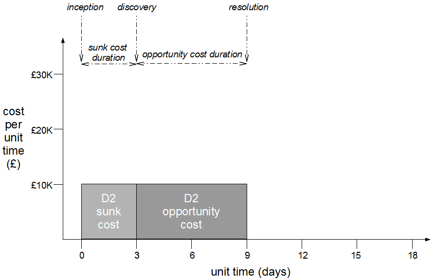
cost per unit time = £10,000
sunk cost = 3 days * £10,000 = £30,000
opportunity cost = 6 days * £10,000 = £60,000
overall cost = sunk cost + opportunity cost = £90,000
When we triage D2 we discover its cost per unit time has decreased to £1,000 per day, meaning its sunk cost is a poor indicator of opportunity cost and its Cost of Delay is lower than expected. Based upon the new 6 day lead time we recommend to the organisation that it defer a D2 fix for at least one release in order to implement pending value-add of greater value than the £12,000 opportunity cost of D2.
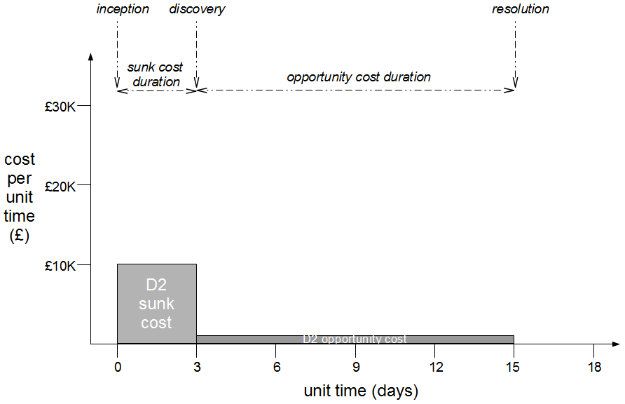
cost per unit time = 3 days * £10,000, 12 days * £1,000
sunk cost = 3 days * £10,000 = £30,000
opportunity cost = 12 days * £1,000 = £12,000
overall cost = sunk cost + opportunity cost = £42,000
The assumption within many IT organisations that risk is directly proportional to rate of change is flawed, as it assumes a constant large batch size. Risk is actually proportional to size of change, and a low release cadence of large changesets is not as effective a risk reduction strategy as a high release cadence of small changesets. Continuous Delivery enables the release of smaller changesets to rapidly release value-add as well as reducing both the probability and cost of defects.