On Tech

Tag: Continuous Delivery levels

The maintenance mode myth

“Over the years, I’ve worked with many organisations who transition live software services into an operations team for maintenance mode. There’s usually talk of being feature complete, of costs needing to come under control, and the operations team being the right people for BAU work. 

It’s all a myth. You’re never feature complete, you’re not measuring the cost of delay, and you’re expecting your operations team to preserve throughput, reliability, and quality on a shoestring budget.

You can ignore opportunity costs, but opportunity costs won’t ignore you.”

Steve Smith

Introduction

Maintenance mode is when a digital service is deemed to be feature complete, and transitioned into BAU maintenance work. Feature development is stopped, and only fixes and security patches are implemented. This usually involves a delivery team handing over their digital service to an operations team, and then the delivery team is disbanded.

Maintenance mode is everywhere that IT as a Cost Centre can be found. It is usually implemented by teams handing over their digital services to the operations team upon feature completion, and then the teams are disbanded. This happens with the Ops Run It operating model, and with You Build It You Run It as well. Its ubiquity can be traced to a myth: 

Maintenance mode by an operations team preserves the same protection for the same financial exposure

This is folklore. Maintenance mode by your operations team might produce lower run costs, but it increases the risk of revenue losses from stagnant features, operational costs from availability issues, and reputational damage from security incidents.

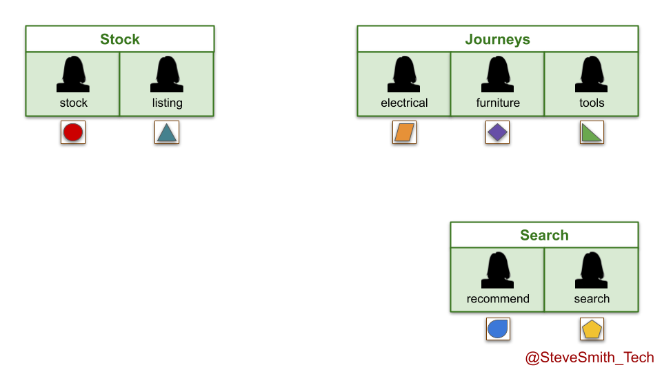
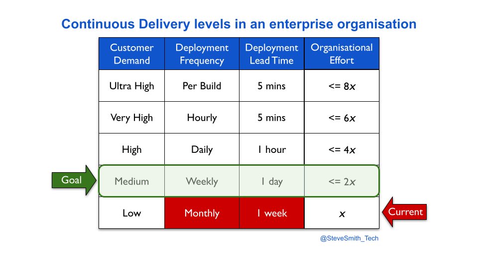
Imagine a retailer DIYers.com, with multiple digital services in multiple product domains. The product teams use You Build It You Run It, and have achieved their Continuous Delivery target measure of daily deployments. There is a high standard of quality and reliability, with incidents rapidly resolved by on-call product team engineers.

DIYers.com digital services are put into maintenance mode with the operations team after three months of live traffic. Product teams are disbanded, and engineers move into newer teams. There is an expected decrease in throughput, from daily to monthly deployments. However, there is also an unexpected decrease in quality and reliability. The operations team handles a higher number of incidents, and takes longer to resolve them than the product teams.

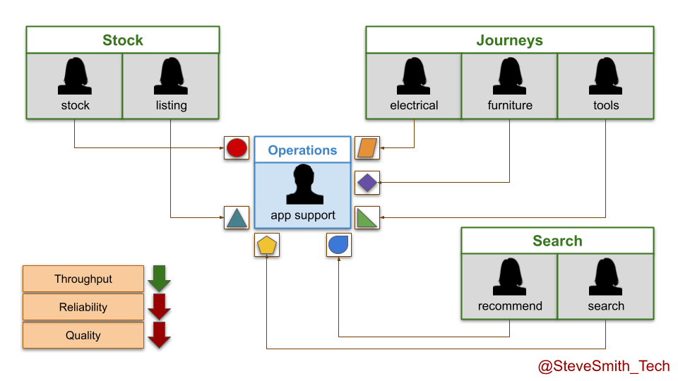
This produces some negative outcomes:

  • Higher operational costs. The reduced run costs from fewer product teams are overshadowed by the financial losses incurred during more frequent and longer periods of DIYers.com website unavailability. 
  • Lower customer revenues. DIYers.com customers are making fewer website orders than before, spending less on merchandise per order, and complaining more about stale website features. 

DIYers.com learned the hard way that maintenance mode by an operations team reduces protection, and increases financial exposure. 

Maintenance mode reduces protection

Maintenance mode by an operations team reduces protection, because it increases deployment lead times.

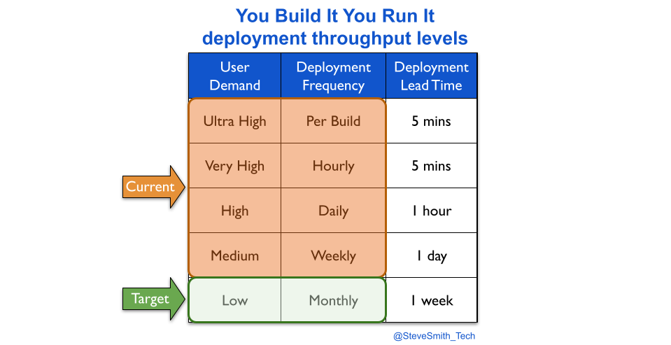
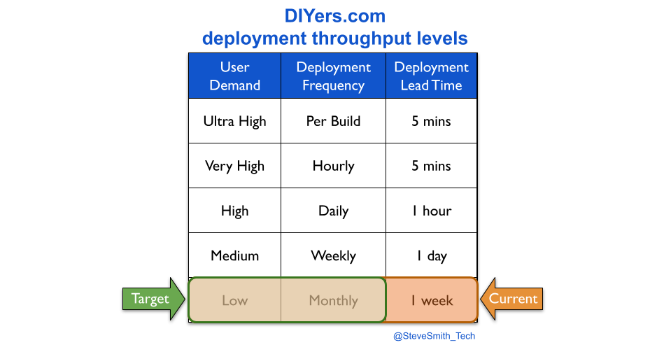
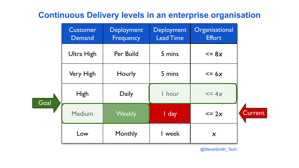
Transitioning a digital service into an operations team means fewer deployments. This can be visualised with deployment throughput levels. A You Build It You Run It transition reduces weekly deployments or more to a likely target measure of monthly deployments.

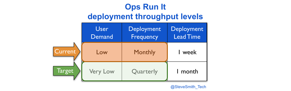
An Ops Run It transition probably reduces monthly deployments to a target measure of quarterly deployments.

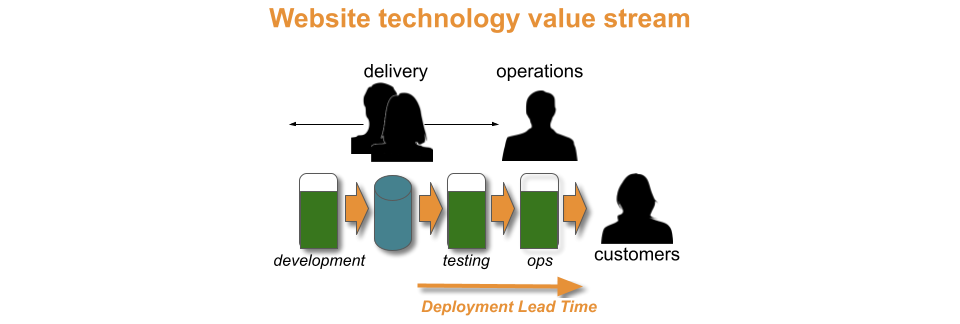
Maintenance mode also results in slower deployments. This happens silently, unless deployment lead time is measured. Reducing deployment frequency creates plenty of slack, and that additional time is consumed by the operations team building, testing, and deploying a digital service from a myriad of codebases, scripts, config files, deployment pipelines, functional tests, etc. 

Longer deployment lead times result in:

  • Lower quality. Less rigour is applied to technical checks, due to the slack available. Feedback loops become enlarged and polluted, as test suites become slower and non-determinism creeps in. Defects and config workarounds are commonplace. 
  • Lower reliability. Less time is available for proactive availability management, due to the BAU maintenance workload. More time is needed to identify and resolve incidents. Faulty alerts, inadequate infrastructure, and major financial losses upon failure become the norm.

This situation worsens at scale. Each digital service inflicted on an operations team adds to their BAU maintenance workload. There is a huge risk of burnout amongst operations analysts, and deployment lead times subsequently rising until monthly deployments become unachievable.

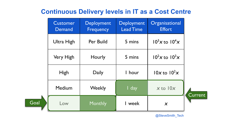
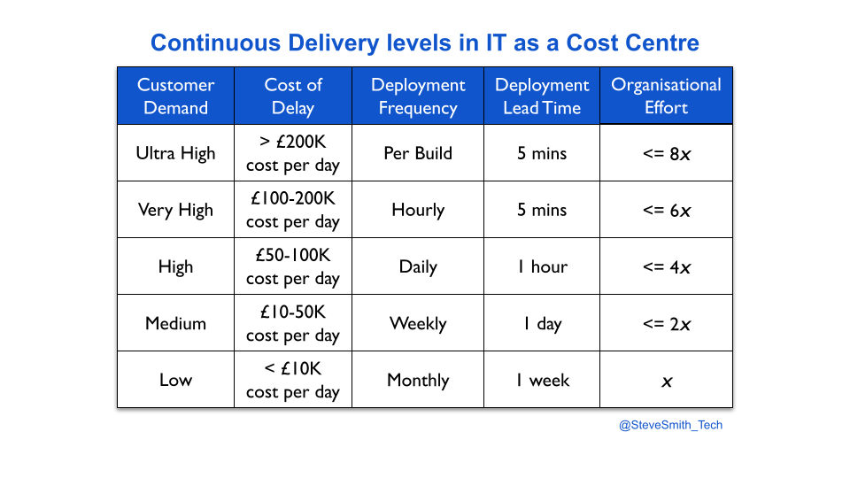
At DIYers.com, the higher operational costs were caused by a loss of protection. The drop from daily to monthly deployments was accompanied by a silent drop in deployment lead time from 1 hour to 1 week. This created opportunities for quality and reliability problems to emerge, and operational costs to increase.

Maintenance mode increases financial exposure

Maintenance mode by an operations team increases financial exposure, because opportunity costs are constant, and unmanageable with long deployment lead times.

Opportunity costs are constant because user needs are unbounded. It is absurd to declare a digital service to be feature complete, because user demand does not magically stop when feature development is stopped. Opportunities to profit from satisfying user needs always exist in a market. 

Maintenance mode is wholly ignorant of opportunity costs. It is an artificial construct, driven by fixed capex budgets. It is true that developing a digital service indefinitely leads to diminishing returns, and expected return on investment could be higher elsewhere. However, a binary decision to end all investment in a digital service squanders any future opportunities to proactively increase revenues. 

Opportunity costs are unmanageable with long deployment times, because a market can move faster than an overworked operations team. The cost of delay can be enormous if days or weeks of effort are needed to build, test, and deploy. Critical opportunities can be missed, such as:

  • Increasing revenues by building a few new features to satisfy a sudden, unforeseeable surge in user demand. 
  • Protecting revenues when a live defect is found, particularly in a key trading period like Black Friday.
  • Protecting revenues, costs, and brand reputation when a zero day security vulnerability is discovered.  

The log4shell security flaw left hundreds of millions of devices vulnerable to arbitrary code execution. It is easy to imagine operations teams worldwide, frantically trying to patch tens of different digital services they did not build themselves, in the face of long deployment lead times and the threat of serious reputational damage. 

At DIYers.com, the lower customer revenues were caused by feature stagnation. The lack of funding for digital services meant customers became dissatisfied with the DIYers.com website, and many of them shopped on competitor websites instead.

Maintenance mode is best performed by product teams

Maintenance mode is best performed by product teams, because they are able to protect the financial exposure of digital services with minimal investment. 

Maintenance mode makes sense, in the abstract. IT as a Cost Centre dictates there are only so many fixed capex budgets per year. In addition, sometimes a digital service lacks the user demand to justify continuing with a dedicated product team. Problems with maintenance mode stem from implementation, not the idea. It can be successful with the following conditions:

  1. Be transparent. Communicate maintenance mode is a consequence of fixed capex budgets, and digital services do not have long-term funding without demonstrating product/market fit e.g. with Net Promoter Score
  2. Transition from Ops Run It to You Build It You Run It. Identify any digital services owned by an operations team, and transition them to product teams for all build and run activities. 
  3. Target the prior deployment lead time. Ensure maintenance mode has a target measure of less frequent deployments and the pre-transition deployment lead time. 
  4. Make product managers accountable. Empower budget holders for product teams to transition digital services in and out of maintenance mode, based on business metrics and funding scenarios. 
  5. Block transition routes to operations teams. Update service management policies to state only self-hosted COTS and back office foundational systems can be run by an operations team. 
  6. Track financial exposure. Retain a sliver of funding for user research into fast moving opportunities, and monitor financial flows in a digital service during normal and abnormal operations. 
  7. Run maintenance mode as background tasks. Empower product teams to retain their live digital services, then transfer those services into sibling teams when funding dries up.  

Maintenance mode works best when product teams run their own digital services. If a team has a live digital service #1 and new funding to develop digital service #2 in the same product domain, they monitor digital service #1 on a daily basis and deploy fixes and patches as necessary. This gives product teams a clear understanding of the pitfalls and responsibilities of running a digital service, and how to do better in the future. 

If funding dictates a product team is disbanded or moved into a different product domain, any digital services owned by that team need to be transferred to a sibling team in the current product domain. This minimises the knowledge sharing burden and BAU maintenance workload for the new product team. It also protects deployment lead times for the existing digital services, and consequently their reliability and quality standards. 

Maintenance mode by product teams requires funding for one permanent product team in each product domain. This drives some positive behaviours in organisational design. It encourages teams working in the same product domain to be sited in the same geographic region, which encourages a stronger culture based on a shared sense of identity. It also makes it easier to reawaken a digital service, as the learning curve is much smaller when sufficient user demand is found to justify further development. 

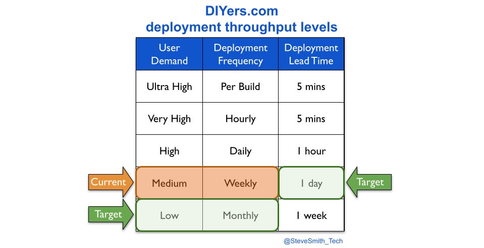
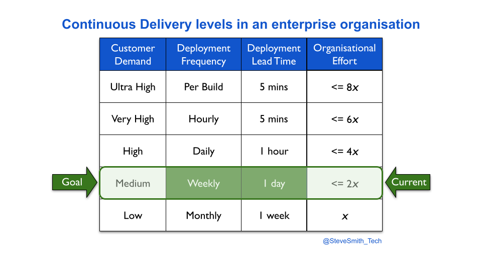
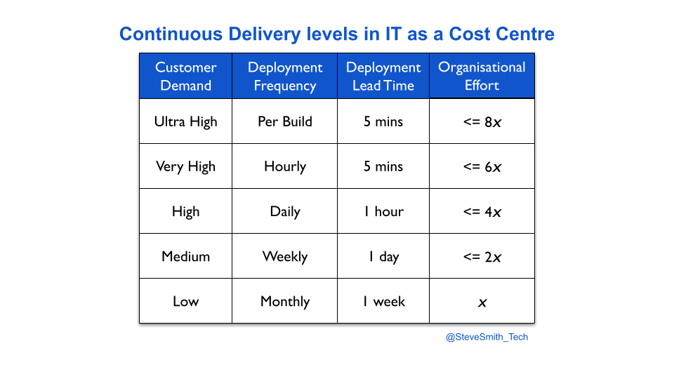
Consider DIYers.com, if maintenance mode was by owned product teams. The organisation-wide target measures for maintenance mode would be expanded, from monthly deployments to monthly deployments performed in under a day.

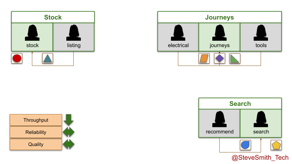
In the stock domain, the listings team is disbanded when funding ends. Its live service is moved into the stock team, and runs in the background indefinitely while development efforts continue on the stock service. The same happens in the search domain, with the recommend service moving into the search team. 

In the journeys domain, the electricals and tools teams both run out of funding. Their live digital services are transferred into the furniture team, which is renamed the journeys team and made accountable for all live digital services there. 

Of course, there is another option for maintenance mode by product teams. If a live digital service is no longer competitive in the marketplace and funding has expired, it can be deleted. That is the true definition of done.

Investing in Continuous Delivery

“Is it possible to overinvest in Continuous Delivery?

The benefits of Continuous Delivery are astonishing, so it’s tempting to say no. Keep on increasing throughput indefinitely, and enjoy the efficiency gains! But that costs time and money, and if you’re already satisfying customer demand… should you keep pushing so hard?

If you’ve already achieved Continuous Delivery, sometimes your organisation should invest its scarce resources elsewhere – for a time. Continuously improve in the fuzzy front end of product development, as well as in technology.”

Steve Smith

TL;DR:

  • Deployment throughput levels describe the effort necessary to implement Continuous Delivery in an enterprise organisation. 
  • Investing in Continuous Delivery means experimenting with technology and organisational changes to find and remove constraints in build, testing, and operational activities.
  • When such a constraint does not exist, it is possible to overinvest in Continuous Delivery beyond the required throughput level.

Introduction

Continuous Delivery means increasing deployment throughput until customer demand is satisfied. It involves radical technology and organisational changes. Accelerate by Dr. Nicole Forsgren et al describes the benefits of Continuous Delivery:

  • A faster time to market, and increased revenues.
  • A substantial improvement in technical quality, and reduced costs.
  • An uptick in profitability, market share, and productivity. 
  • Improved job satisfaction, and less burnout for employees.

If an enterprise organisation has IT as a Cost Centre, funding for Continuous Delivery is usually time-limited and orthogonal to development projects. Discontinuous Delivery and a historic underinvestment in continuous improvement are the starting point.

Continuous Delivery levels provide an estimation heuristic for different levels of deployment throughput versus organisational effort. A product manager might hypothesise their product has to move from monthly to weekly deployments, in order to satisfy customer demand. It can be estimated that implementing weekly deployments would take twice as much effort as monthly deployments.

Once the required throughput level is reached, incremental improvement efforts need to be funded and completed as business as usual. This protects ongoing deployment throughput, and the satisfaction of customer demand. The follow-up question is then how much more time and money to spend on deployment throughput. This can be framed as:

Is it possible to overinvest in Continuous Delivery?

To answer this question, a deeper understanding of how Continuous Delivery happens is necessary.

Investing with a deployment constraint

In an organisation, a product traverses a value stream with a fuzzy front end of design and development activities, and a technology value stream of build, testing, and operational activities. 

With a Theory Of Constraints lens, Discontinuous Delivery is caused by a constraint within the technology value stream. Time and money must be invested in technology and organisational changes from the Continuous Delivery canon, to find and remove that constraint. An example would be from You Build It Ops Run It, where a central operations team cannot keep up with deployment requests from a development team.

The optimal approach to implementing Continuous Delivery is the Improvement Kata. Improvement cycles are run to experiment with different changes. This continues until all constraints in the technology value stream are removed, and the flow of release candidates matches the required throughput level.

The overinvestment question can now be qualified as:

Is it possible to overinvest in Continuous Delivery, once constraints on deployment throughput are removed and customer demand is satisfied?

The answer depends on the amount of time and money to be invested, and where else that investment could be made in the organisation.

Investing without a deployment constraint

Indefinite investment in Continuous Delivery is possible. The deployment frequency and deployment lead time linked to a throughput level are its floor, not its ceiling. For example, a development team at its required throughput level of weekly deployments could push for a one hour deployment lead time.

Deployment lead time strongly correlates with technical quality. An ever-faster deployment lead time tightens up feedback loops, which means defects are found sooner, rework is reduced, and efficiency gains are accrued. The argument for a one hour deployment lead time is to ensure a developer receives feedback on their code commits within the same day, rather than the next working day with a one day deployment lead time. 

Advocating for a one hour deployment lead time that exceeds the required throughput level is wrong, due to: 

  • Context. A one day deployment lead time might mean eight hours waiting for test feedback from an overnight build, before a 30 minute automated deployment to production. Alternatively, it might mean a 30 minute wait for automated tests to complete, before an eight hour manual deployment. A developer might receive actionable feedback on the same day. 
  • Cost. Incremental improvements are insufficient for a one hour deployment lead time. Additional funding is inevitably needed, as radical changes in build, testing, and operational activities are involved. In Lean Manufacturing, this is the difference between kaizen and kaikaku. It is the difference between four minutes refactoring a single test in an eight hour test suite, and four weeks parallelising all those tests into a 30 minute execution time.  
  • Culture. Radical changes necessary for a one hour deployment lead time can encounter strong resistance when customer demand is already satisfied, and there is no unmet business outcome. The lack of business urgency makes it easier for people to refuse changes, such as a change management team declining to switch from a pre-deployment CAB approval to a post-deployment automated audit trail.  
  • Constraints. A one hour deployment lead time exceeding the required throughput level is outside Discontinuous Delivery. There is no constraint to find and remove in the technology value stream. There is instead an upstream constraint in the fuzzy frontend. Time and money would be better invested in business development or product design, rather than Continuous Delivery. Removing the fuzzy frontend constraint could shorten the cycle time for product ideas, and uncover new revenue streams. 

The correlation between deployment lead time and technical quality makes an indefinite investment in Continuous Delivery tempting, but overinvestment is a real possibility. Redirecting continuous improvement efforts at the fuzzy frontend after Continuous Delivery has been achieved is the key to unlocking more customer demand, raising the required throughput level, and creating a whole new justification for funding further Continuous Delivery efforts.

Example – Gardenz

Gardenz is a retailer. It has an ecommerce website that sells garden merchandise. It takes one week to deploy a new website version, and it happens once a month. The product manager estimates weekly deployments of new product features would increase customer sales. 

The Gardenz website is in a state of Discontinuous Delivery, as the required throughput level is unmet. The developers previously needed five days to establish monthly deployments, so ten days is estimated for weekly.

The Gardenz constraint is manual regression testing. It causes so much rework between developers and testers that deployment lead time cannot be less than one week.

The Gardenz developers and testers run improvement cycles to merge into a single delivery team, and replace their manual regression tests with automated functional tests. After fourteen days of effort, a deployment lead time of one day is possible. This allows the website to be deployed once a week, in under a day.

Gardenz has moved up a throughput level to weekly deployments, and the product manager is satisfied. Now they need to decide whether to invest further in daily deployments, beyond customer demand. As weekly deployments took 14 days, 28 days of time and money can be estimated for daily. 

The removal of the testing constraint on weekly deployments causes a planning constraint to emerge for daily deployments. New feature ideas cannot move through product planning faster than two days, no matter whether the deployment lead time is one day, one hour, or one minute. The product manager decides to invest the available time and money into removing the planning constraint. Daily deployments are earmarked for future consideration.

Example – Puzzle Planet

Puzzle Planet is a media publisher. Every month, it sells a range of puzzle print magazines to newsagent resellers. Its magazines come from a fully automated content pipeline. It takes one day for a magazine to be automatically created and published to print distributors. 

The Puzzle Planet content pipeline is in a state of Continuous Delivery. The required throughput level of monthly magazines is met. It took two developers six months to reach a one week content lead time, and a further nine months to exceed the throughput level with a one day content lead time. 

There is no constraint within the content pipeline. The content pipeline also serves a subscription-based Puzzle Planet app for mobile devices, in an attempt to enter the digital puzzle market. Subscribers receive new puzzles each day, and an updated app version every two months. Uptake of the app is limited, and customer demand is unclear.

Puzzle Planet has benefitted from exceeding its required throughput level with a one day content lead time. The content pipeline is highly efficient. It produces high quality puzzles with near-zero mistakes, and handles print distributors with no employee costs. It could theoretically scale up to hundreds of magazine titles. However, a one week content lead time would serve similar purposes.

The problem is the lack of customer demand for the Puzzle Planet app. Digital marketing is the constraint for Puzzle Planet, not its content pipeline or print magazines. An app with few customers and bi-monthly features will struggle in the marketplace, regardless of content updates.

As it stands, the nine months spent on a one day content lead time was an overinvestment in Continuous Delivery. The nine months of funding for the content pipeline could have been invested in digital marketing instead, to better understand customer engagement, retention, and digital revenue opportunities. If more paying customers can be found for the Puzzle Planet app, the one day content lead time could be turned around into a worthy investment.

Acknowledgements

Thanks to Adam Hansrod for his feedback.

Continuous Delivery levels

“When I’m asked how long it’ll take to implement Continuous Delivery, I used to say ‘it depends’. That’s a tough conversation starter for topics as broad as culture, engineering excellence, and urgency.

Now, I use a heuristic that’s a better starter – ‘around twice as much effort than your last step change in deployments’. Give it a try!”

Steve Smith

TL;DR:

  • Continuous Delivery is challenging and time-consuming to implement in enterprise organisations.
  • The author has an estimation heuristic that ties levels of deployment throughput with the maximum organisational effort required.
  • A product manager must choose the required throughput level for their service.
  • Cost Of Delay can be used to calculate a required throughput level.

Introduction

Continuous Delivery is about a team increasing the throughput of its deployments until customer demand is sustainably met. In Accelerate, Dr. Nicole Forsgren et al demonstrate that Continuous Delivery produces:

  • High performance IT. Better throughput, quality, and stability.
  • Superior business outcomes. Twice as likely to exceed profitability, market share, and productivity goals.
  • Improved working conditions. A generative culture, less burnout, and more job satisfaction.

If an enterprise organisation has IT as a Cost Centre, Continuous Delivery is unlikely to happen organically in one delivery team, let alone many. Systemic continuous improvement is incompatible with incentives focussed on project deadlines and cost reduction targets. Separate funding may be required for adopting Continuous Delivery, and approval may depend on an estimate of duration. That can be a difficult conversation, as the pathways to success are unknowable at the outset.

Continuous Delivery means applying a multitude of technology and organisational changes to the unique circumstances of an organisation. An organisation is a complex, adaptive system, in which behaviours emerge from unpredictable interactions between people, teams, and departments. Instead of linear cause and effect, there is a dispositional state representing a set of possibilities at that point in time. The positive and/or negative consequences of a change cannot be predicted, nor the correct sequencing of different changes.

An accurate answer to the duration of a Continuous Delivery programme is impossible upfront. However, an approximate answer is possible. 

Continuous Delivery levels

In Site Reliability Engineering, Betsey Byers et al describe reliability engineering in terms of availability levels. Based on their own experiences, they suggest ‘each additional nine of availability represents an order of magnitude improvement. For example, if a team achieves 99.0% availability with x engineering effort, an increase to 99.9% availability would need a further 10x effort from the exact same team.

In a similar fashion, deployment throughput levels can be established for Continuous Delivery. Deployment throughput is a function of deployment frequency and deployment lead time, and common time units can be defined as different levels. When linked to the relative efforts required for technology and organisational changes, throughput levels can be used as an estimation heuristic.

Based on ten years of author experiences, this heuristic states an increase in deployments to a new level of throughput requires twice as much effort as the previous level. For instance, if two engineers needed two weeks to move their service from monthly to weekly deployments, the same team would need one month of concerted effort for daily deployments.

The optimal approach to implement Continuous Delivery is to use the Improvement Kata. Improvement cycles can be executed to exploit the current possibilities in the dispositional state of the organisation, by experimenting with technology and organisational changes. The direction of travel for the Improvement Kata can be expressed as the throughput level that satisfies customer demand.

A product manager selects a throughput level based on their own risk tolerance. They have to balance the organisational effort of achieving a throughput level with predicted customer demand. The easiest way is to simply choose the next level up from the current deployment throughput, and re-calibrate level selection whenever an improvement cycle in the Improvement Kata is evaluated.

Context matters. These levels will sometimes be inaccurate. The relative organisational effort for a level could be optimistic or pessimistic, depending on the dispositional state of the organisation. However, Continuous Delivery levels will provide an approximate answer of effort immediately, when an exact answer is impossible. 

Quantifying customer demand

A more accurate, slower way to select a deployment throughput level is to quantify customer demand, via the opportunity costs associated with potential features for a service. The opportunity cost of an idea for a new feature can be calculated using Cost of Delay, and the Value Framework by Joshua Arnold et al.

First, an organisation has to establish opportunity cost bands for its deployment throughput levels. The bands are based on the projected impact of Discontinuous Delivery on all services in the organisation. Each service is assessed on its potential revenue and costs, its payment model, its user expectations, and more. 

For example, an organisation attaches a set of opportunity cost bands to its deployment throughput levels, based on an analysis of revenue streams and costs. A team has a service with weekly deployments, and demand akin to a daily opportunity cost of £20K for planned features. It took one week of effort to achieve weekly deployments. The service is due to be rewritten, with an entirely new feature set estimated to be £90K in daily opportunity costs. The product manager selects a throughput level of daily deployments, and the organisational effort is estimated to be 10 weeks.

Acknowledgements

Thanks to Alun Coppack, Dave Farley, and Thierry de Pauw for their feedback.

© 2024 Steve Smith

Theme by Anders NorénUp ↑