“When I’m asked how long it’ll take to implement Continuous Delivery, I used to say ‘it depends’. That’s a tough conversation starter for topics as broad as culture, engineering excellence, and urgency.
Now, I use a heuristic that’s a better starter – ‘around twice as much effort than your last step change in deployments’. Give it a try!”
Steve Smith
TL;DR:
- Continuous Delivery is challenging and time-consuming to implement in enterprise organisations.
- The author has an estimation heuristic that ties levels of deployment throughput with the maximum organisational effort required.
- A product manager must choose the required throughput level for their service.
- Cost Of Delay can be used to calculate a required throughput level.
Introduction
Continuous Delivery is about a team increasing the throughput of its deployments until customer demand is sustainably met. In Accelerate, Dr. Nicole Forsgren et al demonstrate that Continuous Delivery produces:
- High performance IT. Better throughput, quality, and stability.
- Superior business outcomes. Twice as likely to exceed profitability, market share, and productivity goals.
- Improved working conditions. A generative culture, less burnout, and more job satisfaction.
If an enterprise organisation has IT as a Cost Centre, Continuous Delivery is unlikely to happen organically in one delivery team, let alone many. Systemic continuous improvement is incompatible with incentives focussed on project deadlines and cost reduction targets. Separate funding may be required for adopting Continuous Delivery, and approval may depend on an estimate of duration. That can be a difficult conversation, as the pathways to success are unknowable at the outset.
Continuous Delivery means applying a multitude of technology and organisational changes to the unique circumstances of an organisation. An organisation is a complex, adaptive system, in which behaviours emerge from unpredictable interactions between people, teams, and departments. Instead of linear cause and effect, there is a dispositional state representing a set of possibilities at that point in time. The positive and/or negative consequences of a change cannot be predicted, nor the correct sequencing of different changes.
An accurate answer to the duration of a Continuous Delivery programme is impossible upfront. However, an approximate answer is possible.
Continuous Delivery levels
In Site Reliability Engineering, Betsey Byers et al describe reliability engineering in terms of availability levels. Based on their own experiences, they suggest ‘each additional nine of availability represents an order of magnitude improvement. For example, if a team achieves 99.0% availability with x engineering effort, an increase to 99.9% availability would need a further 10x effort from the exact same team.
In a similar fashion, deployment throughput levels can be established for Continuous Delivery. Deployment throughput is a function of deployment frequency and deployment lead time, and common time units can be defined as different levels. When linked to the relative efforts required for technology and organisational changes, throughput levels can be used as an estimation heuristic.
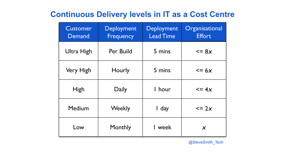
Based on ten years of author experiences, this heuristic states an increase in deployments to a new level of throughput requires twice as much effort as the previous level. For instance, if two engineers needed two weeks to move their service from monthly to weekly deployments, the same team would need one month of concerted effort for daily deployments.
The optimal approach to implement Continuous Delivery is to use the Improvement Kata. Improvement cycles can be executed to exploit the current possibilities in the dispositional state of the organisation, by experimenting with technology and organisational changes. The direction of travel for the Improvement Kata can be expressed as the throughput level that satisfies customer demand.
A product manager selects a throughput level based on their own risk tolerance. They have to balance the organisational effort of achieving a throughput level with predicted customer demand. The easiest way is to simply choose the next level up from the current deployment throughput, and re-calibrate level selection whenever an improvement cycle in the Improvement Kata is evaluated.
Context matters. These levels will sometimes be inaccurate. The relative organisational effort for a level could be optimistic or pessimistic, depending on the dispositional state of the organisation. However, Continuous Delivery levels will provide an approximate answer of effort immediately, when an exact answer is impossible.
Quantifying customer demand
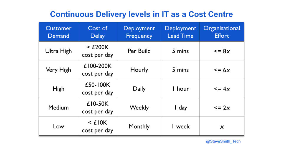
A more accurate, slower way to select a deployment throughput level is to quantify customer demand, via the opportunity costs associated with potential features for a service. The opportunity cost of an idea for a new feature can be calculated using Cost of Delay, and the Value Framework by Joshua Arnold et al.
First, an organisation has to establish opportunity cost bands for its deployment throughput levels. The bands are based on the projected impact of Discontinuous Delivery on all services in the organisation. Each service is assessed on its potential revenue and costs, its payment model, its user expectations, and more.
For example, an organisation attaches a set of opportunity cost bands to its deployment throughput levels, based on an analysis of revenue streams and costs. A team has a service with weekly deployments, and demand akin to a daily opportunity cost of £20K for planned features. It took one week of effort to achieve weekly deployments. The service is due to be rewritten, with an entirely new feature set estimated to be £90K in daily opportunity costs. The product manager selects a throughput level of daily deployments, and the organisational effort is estimated to be 10 weeks.
Acknowledgements
Thanks to Alun Coppack, Dave Farley, and Thierry de Pauw for their feedback.
Recent Comments